
Variables can be either quantitative or qualitative. Quantitative variables are numeric values that count or measure an individual. Qualitative variables are words or categories used to describe a quality of an individual. Qualitative variables are also called categorical variables and can sometimes have numeric responses that represent a category or word. Qualitative or categorical variable – answer is a word or name that describes a quality of the individual. Quantitative or numerical variable – answer is a number (quantity), something that can be counted or measured from the individual. Each type of variable has different graphs, parameters and statistics that you find. Quantitative variables usually have a number line associated with graphical displays. Qualitative variables usually have a category name associated with graphical displays. Examples of quantitative variables are number of people per household, age, height, weight, time (usually things we can count or measure). Examples of qualitative variables are eye color, gender, sports team, yes/no (usually things that we can name). When setting up survey questions it is important to know what statistical questions you would like the data to answer. For example, a company is trying to target the best age group to market a new game. They put out a survey with the ordinal age groupings: baby, toddler, adolescent, teenager, adult, and elderly. We could narrow down a range of ages for, say, teenagers to 13-19, although many 19-year-olds may record their response as an adult. The company wants to run an ad for the new game on television and they realize that 13-year-olds do not watch the same shows nor in the same time slots as 19-year-olds. To narrow down the age range the survey question could have just asked the person’s age. Then the company could look at a graph or average to decide more specifically that 17-year-olds would be the best target audience.
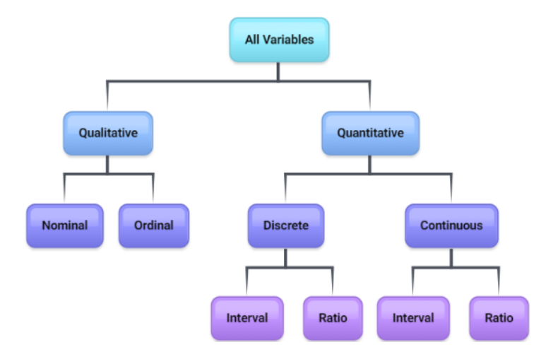
Nominal and ordinal data are qualitative, while interval and ratio data are quantitative.
Likert scales are ordinal in that one can easily see that the larger number corresponds to a higher level of agreeableness. Some people argue that since there is a one-unit difference between the numeric values Likert scales should be interval data. However, the number 1 is just a placeholder for someone that strongly disagrees. There is no way to quantify a one-unit difference between two different subjects that answered 1 or 2 on the scale. For example, one person’s response for strongly disagree could stem from the exact same reasoning behind another person’s response of disagree. People view subjects at different intensities that is not quantifiable.
Quantitative variables are discrete or continuous. This difference will be important later on when we are working with probability. Discrete variables have gaps between points that are countable, usually integers like the number of cars in a parking garage or how many people per household. A continuous variable can take on any value and is measurable, like height, time running a race, distance between two buildings. Usually, just asking yourself if you can count the variable then it is discrete and if you can measure the variable then it is continuous. If you can actually count the number of outcomes (even if you are counting to infinity), then the variable is discrete.
Discrete variables can only take on particular values like integers.
Discrete variables have outcomes you can count.
Continuous variables can take on any value.
Continuous variables have outcomes you can measure.
For example, think of someone’s age. They may report in a survey an integer value like 28 years-old. The person is not exactly 28 years-old though. From the time of their birth to the point in time that the survey respondent recorded, their age is a measurable number in some unit of time. A person’s true age has a decimal place that can keep going as far as the best clock can measure time. It is more convenient to round our age to an integer rather than 28 years 5 months, 8 days, 14 hours, 12 minutes, 27 seconds, 5 milliseconds or as a decimal 28.440206335775. Therefore, age is continuous.
However, a continuous variable like age could be broken into discrete bins, for example, instead of the question asking for a numeric response for a person’s age they could have had discrete age ranges where the survey respondent just checks a box.
When a survey question takes a continuous variable and chunks it into discrete categories, especially categories with different widths, you limit what type of statistics you can do on that data.
Figure 1-2 is a breakdown of the different variable and data types.
If you want to know something about a population, it is often impossible or impractical to examine the entire population. It might be too expensive in terms of time or money to survey the population. It might be impractical: you cannot test all batteries for their length of lifetime because there would not be any batteries left to sell.
When you choose a sample, you want it to be as similar to the population as possible. If you want to test a new painkiller for adults, you would want the sample to include people of different weights, age, etc. so that the sample would represent all the demographics of the population that would potentially take the painkiller. The more similar the sample is to the population, the better our statistical estimates will be in predicting the population parameters.
There are many ways to collect a sample. No sampling technique is perfect, and there is no guarantee that you will collect a representative sample. That is unfortunately the limitation of sampling. However, several techniques can result in samples that give you a semi-accurate picture of the population. Just remember to be aware that the sample may not be representative of the whole population. As an example, you can take a random sample of a group of people that are equally distributed across all income groups, yet by chance, everyone you choose is only in the high-income group. If this happens, it may be a good idea to collect a new sample if you have the time and money.
When setting up a study there are different ways to sample the population of interest. The five main sampling techniques are:
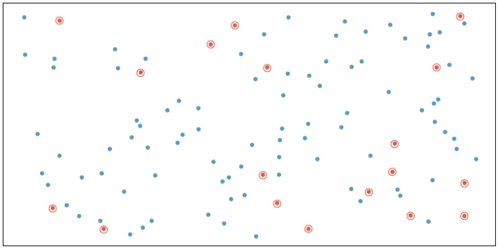
A simple random sample (SRS) means selecting a sample size of n objects from the population so that every sample of the same size n has equal probability of being selected as every other possible sample of the same size from that population. For example, we have a database of all PSU student data and we use a random number generator to randomly select students to receive a questionnaire on the type of transportation they use to get to school. See Figure 1-3. Simple random sampling was used to randomly select the 18 cases.
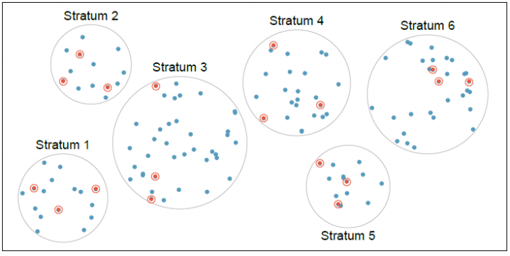
A stratified sample is where the population is split into groups called strata, then a random sample is taken from each stratum. For instance, we divide Portland by ZIP code and then randomly select n registered voters out of each ZIP code. See Figure 1-4. Cases were grouped into strata, then simple random sampling was employed within each stratum.
A cluster sample is where the population is split up into groups called clusters, then one or more clusters are randomly selected and all individuals in the chosen clusters are sampled. Similar to the previous example, we split Portland up by ZIP code, randomly pick 5 ZIP codes and then sample every registered voter in those 5 ZIP codes. See Figure 1-5. Data were binned into nine clusters, three of these clusters were sampled, and all observations within these three clusters were included in the sample.

A systematic sample is where we list the entire population, then randomly pick a starting point at the n th object, and then take every n th value until the sample size is reached. For example, we alphabetize every PSU student, randomly choose the number 7. We would sample the 7 th , 14 th , 21 st , 28 th , 35 th , etc. student.
A convenience sample is picking a sample that is conveniently at hand. For example, asking other students in your statistics course or using social media to take your survey. Most convenience samples will give biased views and are not encouraged.
There are many more types of sampling, snowball, multistage, voluntary, purposive, and quota sampling to name some of the ways to sample from a population. We can also combine the different sampling methods. For example, we could stratify by rural, suburban and urban school districts, then take 3rd grade classrooms as clusters.
The section is an introduction to experimental design. This is a brief introduction on how to design an experiment or a survey so that they are statistically sound. Experimental design is a very involved process, so this is just a small overview.
There are two types of studies:
For instance, if you were to poll students to see if they favor increasing tuition, this would be an observational study since you are asking a question and getting data. Give a patient a medication that lowers their blood pressure. This is an experiment since you are giving the treatment and then getting the data.
Many observational studies involve surveys. A survey uses questions to collect the data and needs to be written so that there is no bias.
Bias is the tendency of a statistic to incorrectly estimate a parameter. There are many ways bias can seep into statistics. Sometimes we don’t ask the correct question, give enough options for answers, survey the wrong people, misinterpret data, sampling or measurement errors, or unrepresentative samples.
In an experiment, there are different options to assign treatments.

No matter which experiment type you conduct, you should also consider the following:
Replication: repetition of an experiment on more than one subject so you can make sure that the sample is large enough to distinguish true effects from random effects. It is also the ability for someone else to duplicate the results of the experiment.
Blind study is where the individual does not know which treatment they are getting or if they are getting the treatment or a placebo.
Double-blind study is where neither the individual nor the researcher knows who is getting the treatment and who is getting the placebo. This is important so that there can be no bias in the results created by either the individual or the researcher.
One last consideration is the time-period that you are collecting the data. There are different time-periods that you can consider.
Cross-sectional study: observational data collected at a single point in time.
Retrospective study: observational data collected from the past using records, interviews, and other similar artifacts.
Prospective (or longitudinal or cohort) study: Subjects are measured from a starting point over time for the occurrence of the condition of interest.
This page titled 1.3: Collecting Data and Sampling Techniques is shared under a CC BY-SA 4.0 license and was authored, remixed, and/or curated by Rachel Webb via source content that was edited to the style and standards of the LibreTexts platform.